- AQH Weekly Deep Dive
- Posts
- Deep Learning for Real-Time Monte Carlo Risk
Deep Learning for Real-Time Monte Carlo Risk
AlgoQuantHub Weekly Deep Dive
Nicholas Burgess
March 06, 2026

Welcome to the Deep Dive!
Each week on The Deep Dive we explore cutting-edge ideas in algorithmic trading, quantitative research, and modern financial engineering. The goal is simple: take current topics used by professional quants and break them down into clear intuition, practical insight, and real implementation examples.
This week we explore how deep learning can transform Monte Carlo pricing into a real-time risk engine. Monte Carlo simulation sits at the heart of modern quantitative finance. It powers the pricing of complex derivatives, credit portfolios, and XVA exposure across large trading books. The challenge is that while Monte Carlo is flexible and accurate, it is computationally expensive. Every risk measure—DV01, CS01, correlation delta, scenario stress—often requires thousands of re-valuations of the model, making real-time risk difficult for complex products.
A powerful new approach is emerging: train a neural network to learn the pricing kernel produced by Monte Carlo. Instead of running expensive simulations every time a price or sensitivity is needed, we generate a large set of simulated market scenarios once, compute the corresponding prices, and train a neural network to learn the pricing function. Modern deep learning frameworks such as PyTorch can run on CUDA GPUs, allowing neural networks to train extremely quickly and evaluate prices in microseconds. The result is a differentiable pricing model capable of producing prices and risk measures in real time.
Bonus content: in this issue we build a neural pricing kernel in PyTorch, demonstrating how Monte Carlo generated training data can be used to teach a neural network the structure of a pricing function. Once trained, we show how automatic differentiation can produce sensitivities such as CS01 and correlation delta instantly, turning a slow simulation engine into a fast real-time risk system.
Table of Contents
Feature Article: Deep Learning for Real-Time Monte Carlo Risk
Monte Carlo simulation is one of the most important tools in quantitative finance. Many financial instruments—especially exotic derivatives and credit portfolio products—have payoff structures that are too complex for closed-form solutions. Instead, quants simulate thousands or millions of possible market paths and estimate the expected payoff numerically. This approach is extremely flexible and can model complicated features such as correlated defaults, stochastic interest rates, and path-dependent payoffs.
However, this flexibility comes with a computational cost. A single price calculation may require thousands of simulated scenarios, and risk calculations often require repeating the entire simulation with small changes to market inputs. For example, computing credit spread sensitivities (CS01) or correlation risk may require dozens or hundreds of Monte Carlo repricings. As a result, large trading books with complex instruments can struggle to produce real-time risk measures.
This is where deep learning provides a compelling alternative. Instead of using Monte Carlo directly for every pricing request, we can use it to generate training data. By simulating a large number of market scenarios and computing the corresponding derivative prices, we can train a neural network to approximate the pricing function itself. In other words, the neural network learns the pricing kernel produced by the Monte Carlo model.
For a comprehensive review of pricing exotic credit and nth-to-default swaps (NTD CDS) see the following reference materials and Excel pricing tools.

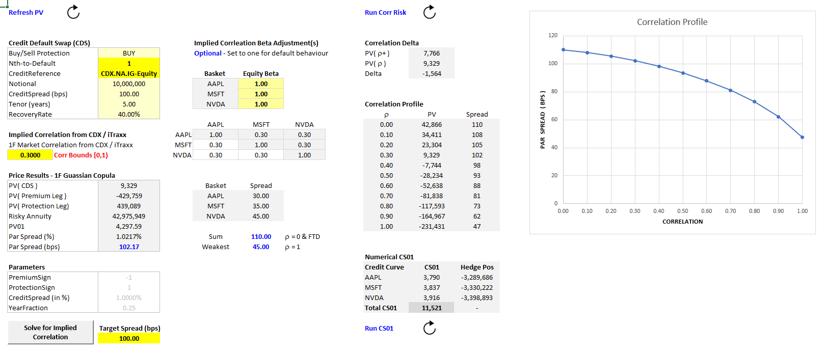
Conceptually, using NTD CDS as an example, the pricing function can be written as,
Price=f( P, S1, S2, … ρ, T )
where
P is a vector of interest-rate swap par spreads used to construct the yield curve
S₁, S₂ … are credit spreads used to calibrate single-name credit curves
ρ represents correlation parameters
T is time to maturity
In a complex credit derivative such as an Nth-to-Default credit default swap, this function can be extremely complicated because it involves correlated default times, survival probabilities, and discounting across many simulated paths. A neural network can learn a highly accurate approximation of this high-dimensional function directly from data.
Once trained, the neural network acts as a surrogate pricing engine. Instead of running a heavy Monte Carlo simulation, the model can evaluate prices almost instantly. Libraries such as PyTorch make this approach particularly attractive because they provide built-in automatic differentiation and GPU support. This means the same model used to produce exotic credit prices can also compute sensitivities such as CS01 or correlation delta automatically.
The workflow therefore becomes:
Monte Carlo simulation → generate training data
Neural network → learn the pricing kernel
Automatic differentiation → produce real-time Greeks
Training the neural network may take time, but it only needs to be performed once. After that, the result is a fast, differentiable pricing engine capable of producing both prices and risk measures in real time.
Recommended Reading
Huge & Savine – Differential Machine Learning
Savine – Modern Computational Finance
Hutchinson, Lo, Poggio – Neural Networks for Option Pricing
Ferguson – Deeply Learning Derivatives
Monte Carlo Methods in Financial Engineering by Paul Glasserman
Monte Carlo Methods in Finance by Peter Jackel
Keywords: Deep Learning, Neural Networks, Monte Carlo, Training Data, Monte Carlo, Real-Time Risk, Exotic Credit Derivatives Modelling, Nth to Default CDS, Algorithmic Trading Research, Quant Finance
Bonus Article: Building a Neural Pricing Kernel in PyTorch
To illustrate the concept, we can build a simple neural pricing model using PyTorch, a popular deep learning framework widely used in quantitative research. PyTorch supports CUDA GPU acceleration, meaning neural networks can train rapidly on modern graphics hardware. While training may take some time depending on the complexity of the model, once the network has learned the pricing function it can evaluate prices almost instantly.
For demonstration purposes we create a simplified toy pricing kernel that mimics the structure of a credit derivative model. The function takes yield curve inputs, credit spreads, and correlation parameters and produces a price. Although simplified, it contains nonlinear rate effects, spread sensitivity, and correlation interaction.
The pricing kernel we aim to learn is
Price = 0.1 ∑ Pi2 + 0.5 ∑ Si + ρ1ρ2
where
Pi are yield curve inputs
Si are credit spreads
ρ are correlation parameters
Using Monte Carlo in practice, we would generate many market scenarios, compute the corresponding derivative prices, and train a neural network to approximate this mapping.
PyTorch Example - Real-Time Risk
Below is a concise well-commented PyTorch example of how to price and compute the real-time risk for exotic credit using nth-to-default CDS as an example using dummy data. Whilst the training may take some time, this only needs to be done once, after which pricing and risk computes in real-time, see below (far-bottom) for the risk results.
import torch
import torch.nn as nn
import torch.optim as optim

# --------------------------------------------------
# 1. Generate training data
# --------------------------------------------------
# Each row represents a market scenario
# Columns:
# 0-4   = yield curve inputs
# 5-9   = credit spreads
# 10-11 = correlation parameters

X_train = torch.rand(5000,12)
X_test  = torch.rand(1000,12)

# --------------------------------------------------
# 2. Toy pricing kernel
# --------------------------------------------------
# In practice this would be a Monte Carlo pricing model

def pricing_kernel(X):

    P = X[:,0:5]      # yield curve inputs
    S = X[:,5:10]     # credit spreads
    rho = X[:,10:12]  # correlations

    price = (
        0.1*(P**2).sum(dim=1, keepdim=True) +   # nonlinear interest-rate effect
        0.5*S.sum(dim=1, keepdim=True) +        # spread contribution
        rho[:,0:1]*rho[:,1:2]                   # correlation interaction
    )

    return price


y_train = pricing_kernel(X_train)
y_test  = pricing_kernel(X_test)

# --------------------------------------------------
# 3. Define neural network
# --------------------------------------------------
# The network will learn the pricing function

class PricingNet(nn.Module):

    def __init__(self):
        super().__init__()

        self.net = nn.Sequential(
            nn.Linear(12,64),
            nn.ReLU(),
            nn.Linear(64,32),
            nn.ReLU(),
            nn.Linear(32,1)
        )

    def forward(self,x):
        return self.net(x)


model = PricingNet()

# --------------------------------------------------
# 4. Training setup
# --------------------------------------------------

criterion = nn.MSELoss()
optimizer = optim.Adam(model.parameters(), lr=0.005)

# --------------------------------------------------
# 5. Train the model
# --------------------------------------------------

for epoch in range(200):

    optimizer.zero_grad()

    predicted = model(X_train)

    loss = criterion(predicted, y_train)

    loss.backward()
    optimizer.step()

    if epoch % 20 == 0:
        with torch.no_grad():
            val_pred = model(X_test)
            val_loss = criterion(val_pred, y_test)

        print(f"Epoch {epoch}, Train Loss: {loss.item():.6f}, Validation Loss: {val_loss.item():.6f}")

# --------------------------------------------------
# 6. Real-time pricing and risk
# --------------------------------------------------

X_new = torch.rand(5,12, requires_grad=True)

prices = model(X_new)

# Automatic differentiation computes sensitivities

prices.sum().backward()

CS01 = X_new.grad[:,5:10]
Correlation_Delta = X_new.grad[:,10:]

print("Prices:", prices.detach().numpy())
print("CS01:", CS01.detach().numpy())
print("Correlation Delta:", Correlation_Delta.detach().numpy())

# --------------------------------------------------
# 7. Accuracy check
# --------------------------------------------------

with torch.no_grad():
    test_pred = model(X_test)

mse = nn.MSELoss()(test_pred, y_test)

pct_error = ((test_pred - y_test).abs()/y_test.abs()).mean()

print("Test MSE:", mse.item())
print("Average percentage error:", pct_error.item()*100)
Once trained, the neural network acts as a fast differentiable approximation of the pricing model. Prices are produced almost instantly, and sensitivities such as CS01 and correlation delta can be computed using automatic differentiation rather than repeated Monte Carlo simulations. We present the real-time risk results below. In large trading systems, this technique can dramatically accelerate portfolio risk calculations, turning heavy simulation engines into efficient real-time analytics tools.
Deep Learning: Real-Time Risk Results
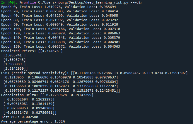
Deep Learning - Real-Time Risk Results
Useful Links
Quant Research
SSRN Research Papers - https://ssrn.com/author=1728976
GitHub Quant Research - https://github.com/nburgessx/QuantResearch
Learn about Financial Markets
Subscribe to my Quant YouTube Channel - https://youtube.com/@AlgoQuantHub
Quant Training & Software - https://payhip.com/AlgoQuantHub
Follow me on Linked-In - https://www.linkedin.com/in/nburgessx/
Explore my Quant Website - https://nicholasburgess.co.uk/
My Quant Book, Low Latency IR Markets - https://github.com/nburgessx/SwapsBook
AlgoQuantHub Newsletters
The Edge
The ‘AQH Weekly Edge’ newsletter for cutting edge algo trading and quant research.
https://bit.ly/AlgoQuantHubEdge
The Deep Dive
Dive deeper into the world of algo trading and quant research with a focus on getting things done for real, includes video content, digital downloads, courses and more.
https://bit.ly/AlgoQuantHubDeepDive
 |  |
Feedback & Requests
I’d love your feedback to help shape future content to best serve your needs. You can reach me at [email protected]