- AQH Weekly Deep Dive
- Posts
- Statistical Edges - Mastering Hypothesis Testing for Pairs Trading
Statistical Edges - Mastering Hypothesis Testing for Pairs Trading
AlgoQuantHub Weekly Deep Dive
Nicholas Burgess
November 14, 2025

Welcome to the Deep Dive!
Here each week on ‘The Deep Dive’ we take a close look at cutting-edge topics on algo trading and quant research.
Last week we discussed the essential algo quant skills needed to succeed in Investment Banks and Hedge Funds — from market intuition and product knowledge, to coding, testing and the math that underpins it all.
This week, we dive into statistical inference and examine the logic behind hypothesis testing, p-values, Type I/II errors, and how these tools help us separate genuine edges from random noise.
Bonus Content, here we dig deeper into stationarity, half-life estimation, and co-integration testing—the statistical core of mean-reversion and pairs-trading strategies.
Table of Contents
Exclusive Algo Quant Store & Discounts
Algo Trading & Quant Research Hub
Get 25% off all purchases at the Algo Quant Store with code 3NBN75MFEA
Feature Article: The Illusion of Certainty – Understanding p-Values and Hypothesis Testing
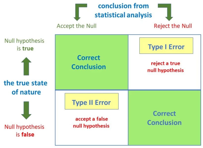
When we perform a statistical test, we step into a curious logical dance. We start by assuming the null hypothesis (H₀) is true—usually something like “there is no relationship” or “the mean difference is zero.” Then, using observed data, we ask: how extreme is this sample if H₀ were true? If it seems very unlikely (a small p-value), we reject H₀. But notice the subtle asymmetry: we never prove the alternative (H₁); we merely find the null improbable under the data. The entire enterprise hinges on testing the data against an assumption we often don’t believe in the first place.
This setup invites two kinds of errors. A Type I error occurs when we wrongly reject a true null—our false alarm rate, α, often set at 0.05. A Type II error happens when we fail to reject a false null—missing a true signal. Reducing α lowers false alarms but raises misses; it’s a trade-off between scepticism and sensitivity. Rejecting H₀ doesn’t mean the effect is “real,” only that our data would be rare if H₀ were true. This nuance is critical in quant finance, where small p-values can mislead when tests are repeated across hundreds of signals or time windows.
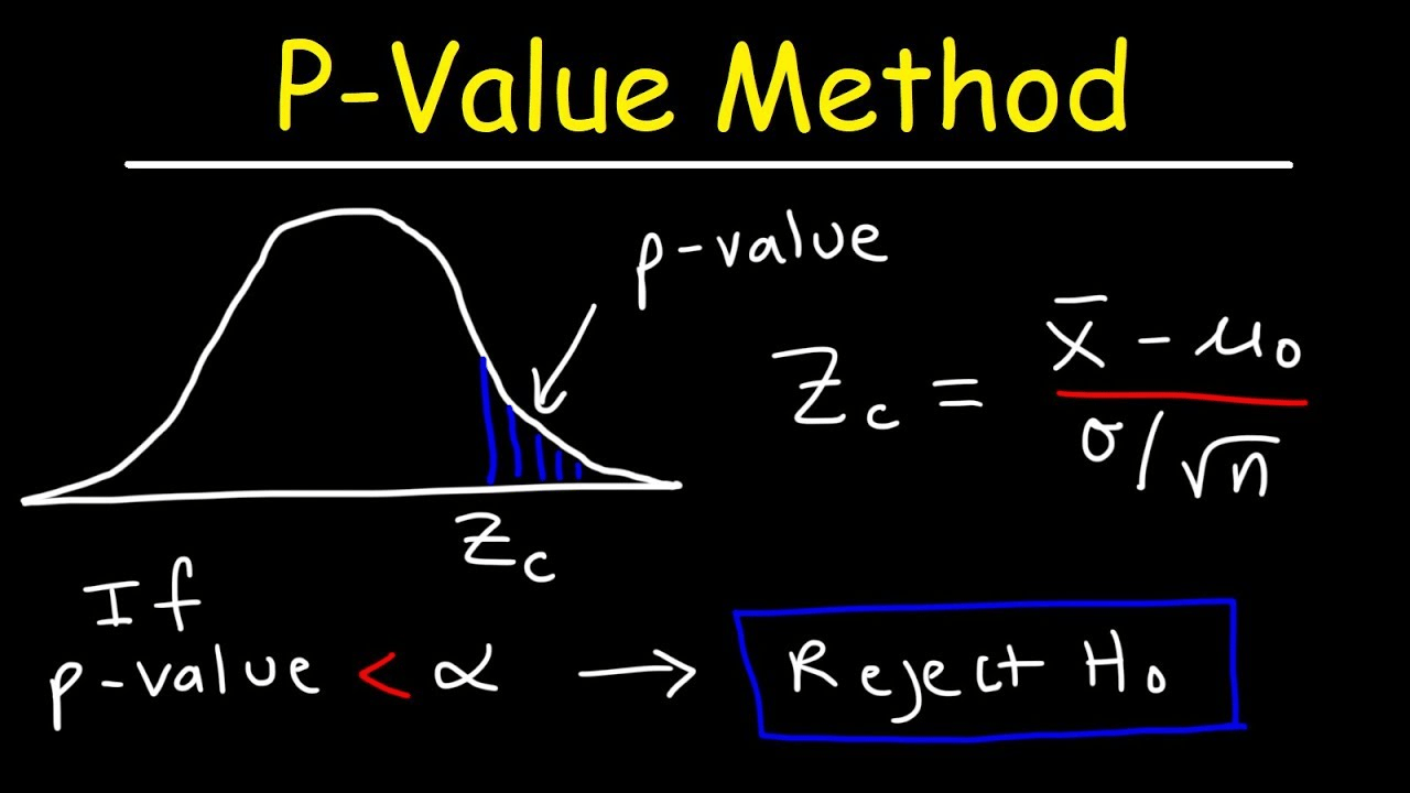
To ground this, consider a test on the mean return of a trading strategy. If the population variance is known or the sample is large (n > 30), we typically assume normality and use a z-test. The test statistic is:

and we compare |z| to the critical value for our chosen α (e.g., 1.96 for 95% confidence). For small samples or unknown variance, we instead rely on the Student’s t-distribution, which fattens the tails to account for uncertainty in variance. The t-statistic looks similar:

where s is the sample standard deviation. The t-distribution converges to the normal as degrees of freedom grow—showing how our “belief” in the underlying variance strengthens with more data.
Before running tests, we need to understand the p-values. The p-value is the probability of observing a test statistic as extreme as—or more extreme than—the one calculated from our sample, assuming H₀ is true. For a t-test, it is derived from the cumulative distribution of the t-distribution with the appropriate degrees of freedom; for a z-test, from the standard normal distribution. It quantifies how surprising the data are under the null hypothesis and is what allows us to decide whether the observed effect is statistically unlikely.
Let’s make this concrete with Python. Suppose we have 30 daily returns of a trading strategy and want to test if the mean return differs from zero:
import numpy as np, scipy.stats as stats

np.random.seed(42)
returns = np.random.normal(0.001, 0.01, 30)  # mean 0.1%, std 1%
t_stat, p_value = stats.ttest_1samp(returns, 0.0)
print(f"t = {t_stat:.3f}, p = {p_value:.4f}")
If p < 0.05, we reject H₀ and claim a statistically significant mean return. But beware: a “significant” result doesn’t mean profitable—it only means the observed mean is unlikely under H₀. Repeat this test across hundreds of strategies and 5% will appear “significant” by chance alone. This is the multiple-testing trap that plagues quantitative research and backtesting.
Hypothesis testing provides structured scepticism rather than certainty—it’s a gatekeeper, not a truth machine. It is a tool to assess whether the observed results are likely to happen if the strategy had no real effect (i.e., under the null hypothesis), quants use p-values to calibrate belief in noisy environments. Alongside cross-validation, out-of-sample testing, and economic reasoning, statistical inference guides signal validation, risk assessment, backtesting, portfolio optimization, anomaly detection, and volatility modelling, helping traders separate genuine edges from random noise.
Recommended Reading
Testing Hypothesis by Minimizing Sum of Errors Type I and Type II, Geeks for Geeks
How to interpret a confusion matrix for a machine learning model, EvidentlyAI
Ultimate Guide to T Tests, GraphPad
Understanding the Confusion Matrix in Machine Learning, Pericchi & Pereira (2013)
Keywords:
Statistics, Machine Learning, p-values, hypothesis testing, null hypothesis, alternative hypothesis, h0, h1, errors, type 1, type 2, false positive, statistical significance, mean return test, cumulative distribution function, PDF, CDF, financial data analysis, statistical inference
Recommended Books for Statistical Arbitrage
The following books are widely regarded as foundational texts for understanding how statistical methods translate into practical, tradable insights.

Bonus Article: The Statistical Tools Behind Pairs Trading
Pairs trading looks deceptively simple: identify two highly related assets, monitor their spread, and trade the divergence. Under the surface, though, the method only works if the statistical structure of that spread behaves in a very specific way. That structure is stationarity.
Why Stationarity Matters?
Before applying any quantitative trading strategy, it is crucial to check if a time series is stationary—meaning its mean, variance, and autocorrelation remain roughly constant over time. Stationarity ensures that patterns we observe historically are statistically meaningful and likely to persist in the short term. The Augmented Dickey-Fuller (ADF) test is the standard tool for this: it tests the null hypothesis H₀ that the series has a unit root (non-stationary). A low p-value allows us to reject H₀, indicating the series is stationary. In practice, stationarity testing is an important filter for candidate securities in mean-reversion and pairs trading strategies: non-stationary series rarely revert predictably and are prone to false trading signals.
Half-Life & Speed of Mean Reversion
For stationary series, we can quantify how quickly they revert to the mean using the half-life of mean reversion.
For an AR(1) process,

the half-life can be computed as,

The half-life indicates the expected number of periods for a deviation from the mean to decay by half. This metric allows traders to prioritize securities:
Short half-life → rapid mean reversion → attractive for fast strategies but may carry higher execution risk or gap exposure.
Long half-life → slower reversion → signals are less actionable.
By combining stationarity and half-life filters, quants can identify securities that revert at a manageable speed, improving the likelihood of capturing predictable moves without excessive operational risk.
Pairs Trading & Engle-Granger Co-Integration
Stationarity testing also underpins pairs trading. Even if two stocks are non-stationary individually, a linear combination may be stationary—a property known as co-integration. The Engle-Granger test implements this: regress one series on another, then test the residuals for stationarity using the ADF test. If the residuals are stationary, the pair is co-integrated and a candidate for mean-reversion trading. Combined with half-life estimation, this allows systematic selection of pairs that revert predictably within an actionable timeframe, balancing profitability and practical execution risk. In the below python code we give an example of how to test for stationarity and co-integration using Exxon Mobile (XOM) and Chevron (CHX) both major players in the oil and gas industry.
import numpy as np
import yfinance as yf
from statsmodels.tsa.stattools import adfuller, coint
from statsmodels.api import OLS, add_constant

# ADF test function: returns True if stationary, False otherwise
def adf_test(series, name="Series", significance=0.05):
    res = adfuller(series, autolag='AIC')
    p_value = res[1]
    is_stationary = p_value < significance
    print(f"\nADF Test for {name}: Statistic={res[0]:.4f}, p-value={p_value:.4f}")
    if is_stationary:
        print(f"Result: Reject H0 → {name} is stationary")
    else:
        print(f"Result: Fail to reject H0 → {name} is non-stationary")
    return is_stationary

# Half-life function: only meaningful for stationary series
def half_life(series):
    x = series.values
    dx = x[1:] - x[:-1]
    x_lag = x[:-1]
    X = add_constant(x_lag)
    est = OLS(dx, X).fit()
    phi_hat = 1 + est.params[1]
    if abs(phi_hat) < 1:
        hl = -np.log(2)/np.log(abs(phi_hat))
        print(f"Estimated phi: {phi_hat:.4f}, Half-life: {hl:.2f} periods")
        return hl
    else:
        print(f"Estimated phi: {phi_hat:.4f}, half-life undefined (non-stationary)")
        return np.nan

# Engle-Granger co-integration test with meaningful output
def engle_granger_test(series1, series2, name1="Series1", name2="Series2", significance=0.05):
    coint_res = coint(series1, series2)
    t_stat, p_value = coint_res[0], coint_res[1]
    print(f"\nEngle-Granger Test for {name1} & {name2}: t-stat={t_stat:.4f}, p-value={p_value:.4f}")
    if p_value < significance:
        print(f"Result: Reject H0 → {name1} and {name2} are co-integrated (stationary spread). Candidate for pairs trading.")
    else:
        print(f"Result: Fail to reject H0 → {name1} and {name2} are not co-integrated. Not suitable for pairs trading.")
    return p_value < significance

if __name__ == "__main__":

    # Fetch example data
    data_xom = yf.download("XOM", start="2024-11-12", end="2025-11-12", auto_adjust=True)["Close"].dropna()
    data_cvx = yf.download("CVX", start="2024-11-12", end="2025-11-12", auto_adjust=True)["Close"].dropna()

    # Test if XOM is stationary and compute half-life only if stationary
    if adf_test(data_xom, "XOM"):
        half_life(data_xom)

    # Test if CVX is stationary and compute half-life only if stationary
    if adf_test(data_cvx, "CVX"):
        half_life(data_cvx)

    # Engle-Granger co-integration test
    engle_granger_test(data_xom, data_cvx, "XOM", "CVX")
Practical Takeaways
Test candidate securities for stationarity using the ADF test before applying mean-reversion strategies.
Use half-life to filter for securities that revert at a realistic speed—fast enough to trade, slow enough to manage risk.
For pairs trading, apply Engle-Granger co-integration, then use half-life to prioritize pairs with actionable mean-reversion.
Avoid formulas and methods that ignore stationarity assumptions—half-life is only meaningful for series that are stationary.
This approach integrates statistical rigor and practical trading intuition, helping quants separate true mean-reverting signals from random noise.
Keywords:
statistics, hypothesis testing, p-values, statistical inference, algorithmic trading, mean reversion, backtesting, trading strategies, financial data, ADF test, Engle-Granger test, co-integration, pairs trading, half-life, stationarity, time series, quantitative research, trading signals, portfolio optimization, volatility modelling, risk management, statistical edges, financial statistics, quant trading, python, financial modelling, market signal filtering
Useful Links
Quant Research
SSRN Research Papers - https://ssrn.com/author=1728976
GitHub Quant Research - https://github.com/nburgessx/QuantResearch
Learn about Financial Markets
Subscribe to my Quant YouTube Channel - https://youtube.com/@AlgoQuantHub
Quant Training & Software - https://payhip.com/AlgoQuantHub
Follow me on Linked-In - https://www.linkedin.com/in/nburgessx/
Explore my Quant Website - https://nicholasburgess.co.uk/
My Quant Book, Low Latency IR Markets - https://github.com/nburgessx/SwapsBook
AlgoQuantHub Newsletters
The Edge
The ‘AQH Weekly Edge’ newsletter for cutting edge algo trading and quant research.
https://bit.ly/AlgoQuantHubEdge
The Deep Dive
Dive deeper into the world of algo trading and quant research with a focus on getting things done for real, includes video content, digital downloads, courses and more.
https://bit.ly/AlgoQuantHubDeepDive
 |  |
Feedback & Requests
I’d love your feedback to help shape future content to best serve your needs. You can reach me at [email protected]