- AQH Weekly Deep Dive
- Posts
- Risk-Neutral Pricing Explained - Replication, Self-Financing Portfolios, No-Arbitrage, Martingales and Convexity Adjustments
Risk-Neutral Pricing Explained - Replication, Self-Financing Portfolios, No-Arbitrage, Martingales and Convexity Adjustments
AlgoQuantHub Weekly Deep Dive
Nicholas Burgess
December 05, 2025
Welcome to the Deep Dive!
Here each week on ‘The Deep Dive’ we take a close look at cutting-edge topics on algo trading and quant research.
Last week, we explored how Monte Carlo with quasi-random number Sobol sequences and Brownian Bridge results in option pricing that converges dramatically faster than traditional pseudo-random simulation.
This week, we examine the full risk-neutral pricing framework from the ground up by linking replication, self-financing portfolios, no-arbitrage conditions, martingales and the role of convexity adjustments. We explain these concepts for traders and quants in clear, everyday language.
Bonus Content, this week we walk through examples of convexity adjustments for Eurodollar Futures, USD SOFR futures and Constant Maturity Swaps (CMS) to show how convexity adjustments arise in real trading and why their economic meaning is often tied directly to replication and choice of numeraire and/or timing and currency adjustments.
Table of Contents
Exclusive Algo Quant Store & Discounts
Algo Trading & Quant Research Hub
Get 25% off all purchases at the Algo Quant Store with code 3NBN75MFEA.


Feature Article: The Risk-Neutral Pricing Framework Explained
"Every derivative can be priced as the cost of creating an arbitrage-free replication portfolio."
This single idea ties together martingales, numeraires, self-financing portfolios, and convexity adjustments.
Replication and Self-Financing Portfolios
Replication sits at the heart of this story. Derivative pricing begins with the assumption that we can construct a replication portfolio of tradable assets that exactly matches the derivative’s payoff, with no arbitrage opportunities. Quants formalize this principle by requiring that the replicating portfolio be self-financing: its value changes only through market movements, perfectly tracking the derivative price over time without the need to add or withdraw capital.
Risk-Neutral World and Numeraires
To formalize pricing, we move into a risk-neutral framework. Here, we choose a tradable asset to serve as the benchmark for pricing and discounting, called the numeraire (e.g., cash account, zero-coupon bond, annuity, swap bond). We then work under the probability measure associated with that numeraire, typically denoted Q.
Martingales and the Martingale Representation Theorem
The numeraire must be tradable and determines the growth of the portfolio (the drift) by adjusting the probabilities of upward and downward moves over time. If we discount the replication payoff using the numeraire, the resulting process becomes a martingale. That is, there is no drift in the discounted process; alternatively, the future value of the discounted process equals its current value. Mathematically, for a process X(t) with t<T,

The martingale property allows us to compute the expected discounted future value of the portfolio as its current price, i.e. the cost of constructing the portfolio. This is formally expressed in the martingale representation theorem (MRT) as,

where V(t) is the value of the derivative, N(t) the numeraire and X(t) the payoff at time t with t<T.
Choosing The Right Numeraire and Measure
Different derivatives call for different numeraires:
If the payoff is linked to cash, use the standard risk-neutral measure Q.
If it depends on a payoff at a specific future date, use the terminal measure Q(T).
For swaps and swaptions, the annuity measure Q(A) or swap measure Q(S) simplifies the dynamics.
Each choice ensures that the corresponding discounted asset becomes a martingale, making risk-neutral valuation straightforward.
Convexity Adjustments
Convexity adjustments arise when the world refuses to be linear. Non-linear payoffs, non-tradable assets, timing differences, and currency (quanto) effects can all break the clean martingale and replication framework. Technically, if a derivative cannot be expressed as a combination of linear tradable assets, the replication portfolio will not perfectly track the derivative price over time.
Typically, convexity adjustments arise when the derivative payoff:
Is a non-linear function of tradable assets (e.g. payoff linked to the square of the stock price say)
Depends on a non-tradable asset (e.g., CMS coupons reference a swap rate)
Involves timing lags (introducing discounting mismatches)
Includes currency adjustments (creating discounting currency mismatches)
Examples include:
CMS coupons are non-linear in forward rates
SOFR futures are not linear in forward rates
Quanto products introduce cross-currency volatility and correlation
In these cases, we apply convexity adjustments — small, mathematically necessary corrections that restore consistency with an arbitrage-free, self-financing portfolio. They ensure the expected discounted payoff still corresponds to something that can be replicated, even if imperfectly.
Putting It All Together
The risk-neutral pricing process follows a clear sequence:
choose a numeraire → replicate the payoff → take the expectation → enter its martingale measure → price the derivative using the MRT formula → make convexity adjustments for non-linear payoffs.
This framework allows traders and quants to price derivatives consistently and know when convexity adjustments are required.
Recommended Reading:
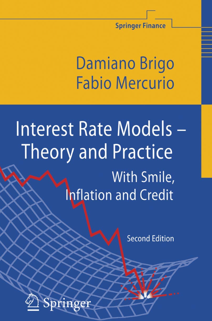
Damiano Brigo / Fabio Mercurio - Interest Rate Models - Theory and Practice
Nicholas Burgess - Convexity Adjustments Made Easy
David Garcia-Lorite / Raul Merino- Convexity Adjustments a la Malliavin
Fabio Mercurio - Valuing Eurodollar-Futures Convexity Adjustments
keywords:
Risk Neutral Pricing, Replication, Self-Financing Portfolio, Arbitrage-Free, Numeraire, Probability Measure, Martingale, Convexity Adjustment
Feature Video: Risk-Neutral Pricing Explained and Applied to American Option Trading
This week’s feature video applies the portfolio replication approach to American option pricing. We discuss what a martingale is in plain English and combine risk-neutral pricing with the Cox Ross Rubenstein (CRR) model or binomial tree to price American Options. It gives an excellent overview of portfolio replication, self-financing, martingales and risk-neutral pricing.
Video Link: Risk-Neutral Pricing Explained
Bonus Article: Convexity Adjustment Examples
Convexity adjustments are most visible in interest rate products where payoffs are non-linear or reference non-tradable assets. We outline here the canonical examples of the Eurodollar Futures convexity adjustment and the USD SOFR futures and Constant Maturity Swap (CMS) convexity adjustments with detailed references and calculations.
Eurodollar Futures
Eurodollar futures are marked-to-market daily, which means gains and losses are realized instantly rather than being discounted to maturity. Forward rates, by contrast, are not realized until settlement and therefore evolve as martingales under the risk-neutral measure after discounting. This difference in settlement timing creates a small but systematic bias: if the short rate is stochastic, then the futures payoff benefits from the correlation between rate shocks and the discount factor, while a forward contract does not. In a lognormal short-rate world, this shows up mathematically as the missing convexity term ½ vol2 * T1 * T2 where T1 and T2 represent the start and end of the underlying forward period. Forward rates require this term because the discount factor is random. Futures do not, because daily marking effectively sets the discounting horizon for each increment to zero.The result is the classic convexity adjustment formula
Ffuture = Fforward + ½ vol2 * T1 * T2
a correction traders add to convert futures-implied rates into forward-implied rates. The proof can be found in classic references such as John Hull, Chapter on Futures Convexity, or Henrard (2005), Eurodollar Futures Convexity Adjustment Revisited, which derive it cleanly using stochastic discount factors and the risk-neutral martingale property.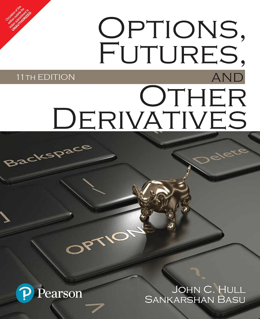
USD SOFR Futures
SOFR futures are quoted in terms of a forward-looking overnight rate but are non-linear in the underlying forward rates. When discounting the expected payoff using the risk-free numeraire, this non-linearity introduces a small difference between the expected futures payoff and the forward rate, which is corrected using a convexity adjustment. Traders often interpret this adjustment as a correction between futures-implied rates and forward rates, while quants derive it formally using the martingale measure and stochastic calculus. For the convexity adjustment, see Valuing Eurodollar-Futures Convexity Adjustments.Constant Maturity Swaps
CMS coupons reference a swap rate, which is not a directly tradable asset. Since the replication portfolio cannot perfectly hedge a swap rate payoff, a convexity adjustment is required to ensure an arbitrage-free valuation. The adjustment accounts for the non-linear relationship between the CMS rate and the underlying zero-coupon bonds or forward rates. Without this correction, pricing and hedging would systematically misestimate expected payoffs. For the convexity adjustment, see Convexity adjustment for constant maturity swaps in a multi-curve framework.
These examples illustrate the practical importance of convexity adjustments: whenever the derivative payoff is non-linear, depends on non-tradable assets, or involves timing/currency effects, a careful adjustment is necessary to maintain a self-financing, arbitrage-free replication framework.
Keywords:
Portfolio Replication, Self-Financing, Arbitrage-Free, Martingale, Measures, Tradable Assets, Risk-Neutral Pricing, Derivatives, Linear Payoffs, Non-Linear Payoffs, Convexity Adjustments
Useful Links
Quant Research
SSRN Research Papers - https://ssrn.com/author=1728976
GitHub Quant Research - https://github.com/nburgessx/QuantResearch
Learn about Financial Markets
Subscribe to my Quant YouTube Channel - https://youtube.com/@AlgoQuantHub
Quant Training & Software - https://payhip.com/AlgoQuantHub
Follow me on Linked-In - https://www.linkedin.com/in/nburgessx/
Explore my Quant Website - https://nicholasburgess.co.uk/
My Quant Book, Low Latency IR Markets - https://github.com/nburgessx/SwapsBook
AlgoQuantHub Newsletters
The Edge
The ‘AQH Weekly Edge’ newsletter for cutting edge algo trading and quant research.
https://bit.ly/AlgoQuantHubEdge
The Deep Dive
Dive deeper into the world of algo trading and quant research with a focus on getting things done for real, includes video content, digital downloads, courses and more.
https://bit.ly/AlgoQuantHubDeepDive
 |  |
Feedback & Requests
I’d love your feedback to help shape future content to best serve your needs. You can reach me at [email protected]