- AQH Weekly Deep Dive
- Posts
- Monte Carlo for Exotic Option Pricing
Monte Carlo for Exotic Option Pricing
AlgoQuantHub Weekly Deep Dive
Nicholas Burgess
August 22, 2025

Welcome to the Deep Dive!
Here each week on ‘The Deep Dive’ we take a close look at cutting-edge topics on algo trading and quant research.
Last week, we presented a low-risk options trading strategy where we sold put options on reputable stocks for income generation to get paid to buy stocks at a discount. If assigned we can sell covered calls to both exit the position and generate additional income. This week, we outline how to use Monte Carlo Simulation to price vanilla and exotic options.
Bonus content, we provide examples of how to price options using the Monte Carlo approach in both C++ and Python. To demo the robustness of the approach, we compare and test price results against the well-known Black-Scholes formula for European option pricing.
Table of Contents
Exclusive Quant Discounts
Get 25% off all purchases at AlgoQuantHub’s digital store with code 3NBN75MFEA
Feature Article: Monte Carlo Option Pricing — A Powerful Quantitative Tool
Monte Carlo simulation is a cornerstone technique in quantitative finance for pricing complex financial derivatives, especially where closed-form solutions do not exist or are difficult to obtain. At its core lies the idea of simulating numerous possible future paths for the underlying asset’s price—typically modeled by a stochastic process such as Geometric Brownian Motion (GBM)—and then computing discounted expected payoffs across these paths under the risk-neutral measure.
The GBM model allows us to estimate or predict future stock paths and is used for derivative pricing, risk management, trading strategy backtesting and forecasting. GBM describes the evolution of the stock price S via a stochastic differential equation (SDE) under the real-world measure P,
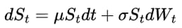
Geometric Brownian Motion SDE
where μ is drift, σ is volatility, and Wt is a Brownian motion. The solution to this SDE can be transformed into an expression that simulates stock prices at any future time t (see resources section below for more info) for a given standard normal random variable Z,
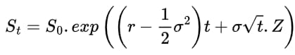
Solution to GBM SDE
The resulting expression operates under the risk-neutral measure Q, where St is a martingale. Importantly, this means the fair price of any derivative is its discounted expected payoff—this is foundational to the risk-neutral pricing framework. Using P(0,t) to represent the discount factor, we write this as,
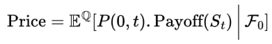
Martingale Representation Theorem
The final result is that we can price derivates by computing their discounted payoffs using a modest number of simulated normal random variates Z and then taking the average.
Monte Carlo simulations excel in versatility and intuitiveness. They easily extend to path-dependent payoffs such as Asian and barrier options, where other pricing methods struggle. While American options—due to early exercise features—require more specialized approaches like finite difference PDEs or binomial trees, regression techniques such as Longstaff-Schwartz provide Monte Carlo-compatible solutions. Monte Carlo is a hallmark tool in quantitative finance due to its conceptual clarity and broad applicability in pricing and risk management.
Option Pricing Training & Resources
Advanced Pricing Tools - by AlgoQuantHub
European Option Pricing - Guide and Excel workbook.
Monte Carlo Simulation for Option Pricing - Theory & Practice Guide
Comes with Excel Workbook, C++ and Python Code for Option Pricing
 MC Simulation Theory & Practice | 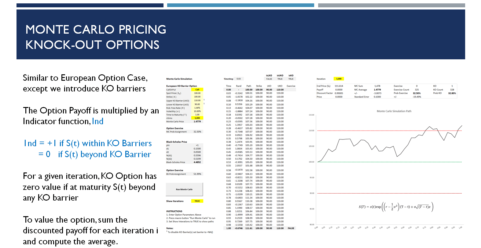 Double KO Barrier Option Pricing |
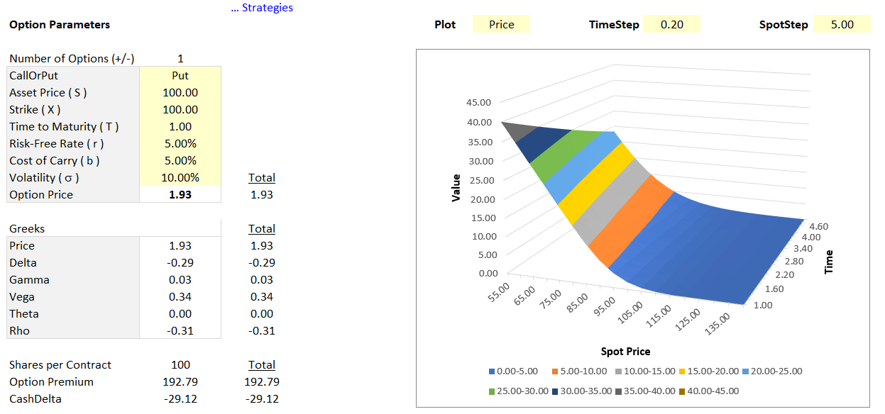 European Option Pricing & Greeks | 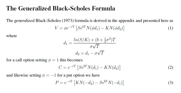 Generalized Black Scholes Formulas |
Recommended Reading
Monte Carlo Methods in Financial Engineering by Paul Glasserman
Monte Carlo Methods in Finance by Peter Jackel
 |  |
Keywords
Derivatives, Options, Pricing, Monte Carlo, Simulation, Forecasting, Martingale, GBM, SDE, Expectations, Discount Factor, Payoff, Real-World Measure, Girsanov’s Theorem, Risk-Neutral Measure, Arbitrage-Free
Bonus Content: Monte Carlo Option Pricing in Practice with C++ and Python
To bring the theory to life, consider the following concise C++ implementation of Monte Carlo pricing for European options. The code simulates terminal prices using GBM under the risk-neutral measure, with the Mersenne Twister RNG generating standard normal draws. The Black-Scholes analytical price serves as a benchmark.
While the C++ native Mersenne Twister Random Number Generator (RNG) works well for many tasks, advanced quant users should consider the Sobol Brownian Bridge RNG available from opensource libraries such as QuantLib. These quasi-random sequences improve convergence significantly—often requiring significantly less simulations (e.g., 5,000 vs 20,000) to achieve the same accuracy.
The Black-Scholes formula uses the normal cumulative distribution function (CDF), efficiently implemented via the error function (erf). This approximation provides accurate and rapid calculations of the European option price’s theoretical benchmark.
Monte Carlo’s strength extends far beyond vanilla options, enabling pricing of path-dependent and exotic derivatives where analytic formulas fail. However, care must be taken with American options, where early exercise features pose challenges; Monte Carlo methods can be adapted via regression-based approaches like Longstaff-Schwartz to handle such complex features.
C++ Code: European Option Pricing using MC Simulation
Below we present a short and fully-functional Monte Carlo option pricing C++ code. The code prices a European option using numerical Monte Carlo simulation and compares simulated results to the exact result from the closed-form Black-Scholes solution. To run simply click-here and select run on the menu-bar.
Random Number Generation
MC simulation requires that we generate random numbers, we do this using the C++ native Mersenne Twister random number generator as shown below.
#include <random>
using namespace std;

// Initialize Mersenne Twister RNG with fixed seed
mt19937 generator(123456);
normal_distribution<double> normsdist(0, 1);

// Generate a Random Number
double z = normsdist(generator);
Normal Cumulative Distribution Function (Normal CDF)
The Black-Scholes formula requires the compuation of the standard normal cumulative distribution function (Normal CDF), which we can compute using the error function (erf) from the header #include <cmath> as shown below.
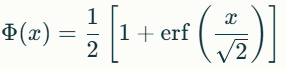
Standard Normal CDF
Black-Scholes Formula
The Monte Carlo pricing routine works for both vanilla and exotic options. To test the pricing routine we price European call and put options using the Black-Scholes formula, which has an exact closed-form solution. We compare the Monte Carlo price results with the analytical solution from the Black-Scholes formula, note we set the indicator function phi to +1 for a call and -1 for a put option.

Black-Scholes Formula
Monte Carlo Results
The error between the Monte Carlo simulated result and the closed-form exact solution is determined by the sample standard deviation with the sample size N equal to the number of simulations. This is called the standard error and is calculated as SE = vol / sqrt(N). It can be used to form a confidence interval (CI) as follows CI = V ± z . SE, where z is the z-score or critical value from the normal distribution e.g. for a 95% confidence interval we have z = ±1.9599.
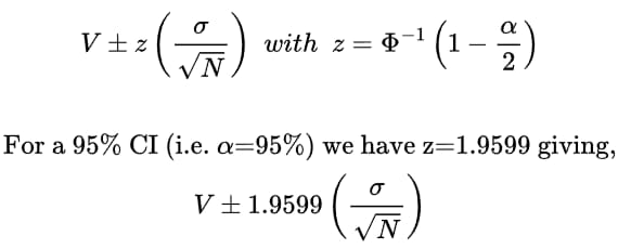
Monte Carlo Confidence Interval
Running the C++ Code
Finally, I present the C++ code for the Monte Carlo code below, which has been preloaded on a free cloud-based C++ compiler. To run click-here and press run on the menu-bar.
#include <iostream>
#include <cmath>
#include <random>
using namespace std;

// Normal CDF using Error Function, erf
double norm_cdf(double x)
{
    return 0.5 * (1 + erf(x / sqrt(2)));
}

// Enum for option type
enum OptionType { Call, Put };

// Black-Scholes formula for European options
// s0 = initial stock price, k = strike, r = interest rate
// v = implied volatility, t = time to expiry (years)
double blackscholes(OptionType type, double s0, double k, double r, double v, double t)
{
    double d1 = (log(s0/k) + (r + 0.5*v*v) * t) / (v*sqrt(t));
    double d2 = d1 - v * sqrt(t);
    double sign = (type == Call) ? 1.0 : -1.0;
    double nd1 = norm_cdf(sign * d1);
    double nd2 = norm_cdf(sign * d2);
    return sign * (s0 * nd1 - k * exp(-r*t) * nd2);
}

// Monte Carlo pricing of European option
double montecarlo(OptionType type, double s0, double k, double r, double v, double t, int nSims = 10000)
{
    // Mersenne Twister RNG with fixed seed
    mt19937 generator(123456);
    normal_distribution<double> normsdist(0, 1);

    // Run Monte Carlo Simulations
    double sign = (type == Call) ? 1.0 : -1.0;
    double price = 0.0;
    for (int i = 1; i <= nSims; ++i)
    {
        // Generate Standard Normal Random Number, z
        double z = normsdist(generator);
        // Use GBM for Stock Price at Time t
        double st = s0 * exp((r - 0.5*v*v) * t + v*sqrt(t)*z);
        double payoff = max(sign * (st - k), 0.0);
        // Martingale Price equals Discounted Payoff
        price += payoff * exp(-r*t);
    }
    // Average Price
    return price / nSims;
}

int main()
{
    // European Call, S=100, K=100, r=1%, vol=10%, t=1 Year
    // Expected Price: 4.485236
    double bs = blackscholes(Call, 100, 100, 0.01, 0.1, 1.0);
    double mc = montecarlo(Call, 100, 100, 0.01, 0.1, 1.0, 20000);
    printf("%s%.6f\n", "Monte Carlo Price: ", mc);
    printf("%s%.6f\n", "Black-Scholes Price: ", bs);
    return 0;
}
Python
The equivalent code in Python is shown below.
# Geometric Brownian Motion simulation & Monte Carlo option pricing notebook
import numpy as np
import matplotlib.pyplot as plt
from scipy.stats import norm
from scipy.stats import lognorm

# Black-Scholes analytic price
def black_scholes_price(call_put_flag, S0, K, r, sigma, T):
    d1 = (np.log(S0 / K) + (r + 0.5 * sigma**2)*T) / (sigma * np.sqrt(T))
    d2 = d1 - sigma * np.sqrt(T)
    if call_put_flag == 'call':
        price = S0 * norm.cdf(d1) - K * np.exp(-r*T) * norm.cdf(d2)
    else:
        price = K * np.exp(-r*T) * norm.cdf(-d2) - S0 * norm.cdf(-d1)
    return price

# Monte Carlo simulation of future price S(T) under risk-neutral GBM
def simulate_gbm(S0, r, sigma, T, nSims, seed=12345):
    np.random.seed(seed)
    Z = np.random.normal(size=nSims)
    ST = S0 * np.exp((r - 0.5 * sigma**2)*T + sigma * np.sqrt(T) * Z)
    return ST

# Monte Carlo pricing for European options
def monte_carlo_price(call_put_flag, S0, K, r, sigma, T, nSims):
    ST = simulate_gbm(S0, r, sigma, T, nSims)
    if call_put_flag == 'call':
        payoffs = np.maximum(ST - K, 0)
    else:
        payoffs = np.maximum(K - ST, 0)
    discounted_payoff = np.exp(-r * T) * payoffs
    price = discounted_payoff.mean()
    std_error = discounted_payoff.std() / np.sqrt(nSims)
    return price, std_error

# European Option Parameters
S0 = 100      # initial stock price
K = 100       # strike price
r = 0.01      # risk-free rate
sigma = 0.1   # volatility
T = 1.0       # time to maturity
nSims = 10000

# Compute Black-Scholes price
bs_price_call = black_scholes_price('call', S0, K, r, sigma, T)
print(f"Black-Scholes call price: {bs_price_call:.6f}")

# Compute Monte Carlo price and standard error
mc_price, standard_error = monte_carlo_price('call', S0, K, r, sigma, T, n)
print(f"Monte Carlo price with {nSims} simulations: {mc_price:.6f} ± {standard_error:.6f}")
Monte Carlo Simulation Results
Keywords
Derivatives, Option Pricing, European, Vanilla, Exotics, Monte Carlo, Simulation, Black-Scholes, Closed-Form, Analytical, Solution, Random Number Generators, Mersenne Twister, Sobol Brownian Bridge, Normal Cumuluative Distribution Function, CDF, Error Function, Programming, C++, CPlusPlus, Python, Standard Error
Useful Links
Quant Research
SSRN Research Papers - https://ssrn.com/author=1728976
GitHub Quant Research - https://github.com/nburgessx/QuantResearch
Learn about Financial Markets
Subscribe to my Quant YouTube Channel - https://youtube.com/@AlgoQuantHub
Quant Training & Software - https://payhip.com/AlgoQuantHub
Follow me on Linked-In - https://www.linkedin.com/in/nburgessx/
Explore my Quant Website - https://nicholasburgess.co.uk/
My Quant Book, Low Latency IR Markets - https://github.com/nburgessx/SwapsBook
AlgoQuantHub Newsletters
The Edge
The ‘AQH Weekly Edge’ newsletter for cutting edge algo trading and quant research.
https://bit.ly/AlgoQuantHubEdge
The Deep Dive
Dive deeper into the world of algo trading and quant research with a focus on getting things done for real, includes video content, digital downloads, courses and more.
https://bit.ly/AlgoQuantHubDeepDive
 |  |
Feedback & Requests
I’d love your feedback to help shape future content to best serve your needs. You can reach me at [email protected]